TLDR: I speak about computer vision, I start by playing with images and build on top of it to introduce this field and we finish by showing how to detect corners in an image using Harris.

This is part 1 of the series, i don’t know how many there will be, but know I want another one on the derivation of Harris and another one on sift.

Assumption: You should know a bit of Numpy indexing and probably Python.

What is Computer Vision?

This semester at uni, I got a lecture called “Vision Algorithms for Mobile Robotics” and I want to walk you through it.
First, let’s distinguish between computer vision and computer graphics:

1. Computer Vision: Use a computer to analyze images.
2. Computer Graphics: Use a computer to create images.

We will focus on the former. If you want to read more, I was recommended “Introduction to autonomous mobile robots, 2nd Edition” by R. Siegwart, I.R. Nourbakhsh, and D. Scaramuzza.

What can we do with it ?

Well, a lot actually, we can reconstruct entire 3D spaces using only images, we can find similar images, recognize places and so on.

First and foremost

Let’s install the necessary packages:

1
2
3
4
5
6

conda create -n cv python=3.12
conda activate cv
pip install opencv-python
conda install scipy
conda install pooch
conda install matplotlib

And now

1
2
3
4
5
6

import cv2 as cv
import scipy as sp
import matplotlib.pyplot as plt
img = sp.datasets.ascent()
cv.imshow("Display window", img)
cv.waitKey(0)

If everything went fine, you should see a staircase with two people.

We are going to work on that picture. Usually, computer vision people like to work on a picture of Lenna a playboy model used in some examples, but this is not considered appropriate anymore, which I absolutely agree with. Therefore you’ll see the staircase instead.

Let’s dive

We are going to highlight fast changes in adjacent pixels. Because a pixel has 8 neighbors (counting diagonal) we can choose which pixel to compare to. A fast way to do it by shifting an image and then subtracting the original image and the shifted one ! The direction of the shift indicates the pixels we want to compare to. By the way, we are going to use black and white images, so the pixel value is between 0 and 255. However, you can also sum up the differences between the 3 channels.

1
2
3
4
5
6
7
8
9

OFFSET = 1 
# Copy img
# Add a row (512 pixels) with a value of 0's on top of the img.
img1 = np.r_[np.zeros((OFFSET,512)), img]
# slice the picture to a shape of 512x512 (original image shape)
img1 = img1[: img.shape[0], : img.shape[1]]
diff_ver = img1-img
plt.imshow(diff_ver,cmap='grey')
plt.show()

What the code does is the following:

1. Copy the image
2. Add a row of 0’s on top of the image
3. Slice the image to the original shape
4. Compute the difference between the two images
5. Show the image

As we can see below, this process of finding rapid changes in neighboring pixels highlights the edges present in the picture.

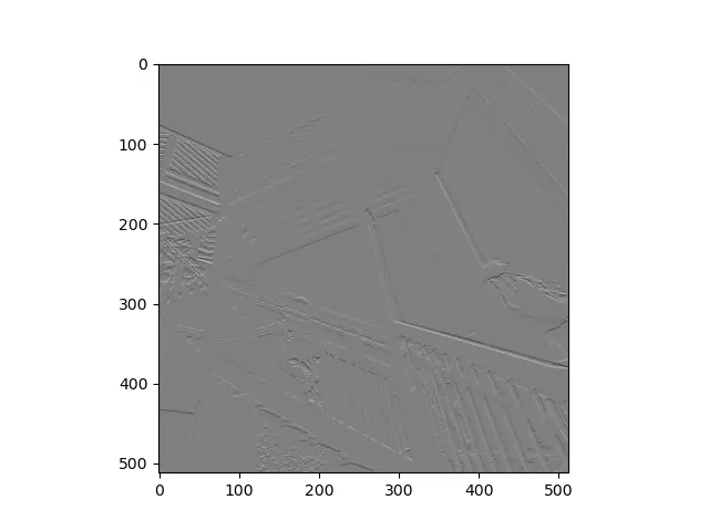
We can do the same by adding a column on the left instead of a row on the top, as we previously did.

1
2
3
4
5
6

# Notice the change in the first line
img1 = np.c_[np.zeros((512,OFFSET)), img]
img1 = img1[: img.shape[0], : img.shape[1]]
diff_hor = img1-img
plt.imshow(diff_hor, cmap='grey')
plt.show()

If you are running the code alongside, you might have noticed that diff_ver and diff_hor are slightly different. Let’s think about what we computed. In the first diff, we added a row, then we computed the pixel-wise differences this is equivalent to computing \(I_{diff}(x,y) = I(x,y)-I(x,y+1) \). Where \(I\) is the image Intensity corresponding to the \(x,y\) coordinates. In the second case we added a column, therefore the \(+1\) is added to the \(x\) instead. i.e. \(I_{diff}(x,y) = I(x,y)-I(x+1,y) \).

Now, how to do it efficiently ?
Obviously by using some libraries but also by using convolutions.

Introducing the convolution with a simple example

Convolution is an operator such as + or -. We compute convolution between signals, and be prepared for the big revelation, an image is a signal !
Bruh WTF!
Yup, I said the same! A (discrete) signal is just an array of numbers, and an image is exactly that, but in 2D. We will start with something simpler than a 2D signal, and build up. Let’s say you have a 1D signal \(S(t)\) where \(t\) is the time ranging from \(0\) to \(8\) (arbitrary chosen). \(S(t) = [1,2,3,4,4,3,2,1]\), we could do the same as we did with the images and subtract \(S(t_k) - S(t_{k+1})\) this would give us :
\([-1 ,-1,-1,0,1,1,1]\).

Now let’s introduce the convolution formally and see how it related to what we have done before: \(\ast\) is the convolution operator and equation (1) is the definition of the convolution.

\begin{align} (A \ast B)[t_k] = \green{\sum_{m}} A[m] \cdot B[t_k-m] \end{align}

\begin{align} S(t) \ast [\blue{\text{-}1},\red{1}] =& [1,2,3,4,4,3,2,1] \ast [\blue{\text{-}1},\red{1}] \\ =&[ \underbrace{1\cdot\red{1} + 2\cdot\blue{\text{-}1},}_{\text{\green{first sum}}} \\ &2\cdot\red{1} + 3\cdot\blue{\text{-}1}, \\ &3\cdot\red{1} + 4\cdot\blue{\text{-}1}, \\ &4\cdot\red{1} + 3\cdot\blue{\text{-}1}, \\ &3\cdot\red{1} + 2\cdot\blue{\text{-}1}, \\ &2\cdot\red{1} + 1\cdot\blue{\text{-}1}] \\ =& [\text{-}1,\text{-}1,\text{-}1,0,1,1,1] \end{align}

Notice how we flipped the second signal, we computed the first result as \(S_1 \cdot \red{B_2} \green{+} S_2 \cdot \blue{B_1}\) therefore swapping \(\red{B_2}\) and \(\blue{B_1}\). We can do all sort of things using convolution on our image, due to an image being a 2D discrete signal !

Smooth bro!

Let’s try something else, what about smoothing the image ? How would you do it ? You would take the average of a region, i.e. You would compute a pixel as the mean of it’s adjacent pixels. Therefore, you would sum the pixel and divide by the number of pixels you took in the neighborhood. These operations might ring a bell, it’s the one involved in the convolution’s definition. We can try to rewrite our idea into a convolution: Instead of dividing by 1/n after the sum, we can multiply every pixel by 1/n and then sum it’s the same and this is writable using convolution !

\begin{align} I_{smooth}(x,y) &= \frac{1}{9}\sum_{u= -1}^1\sum_{v=-1}^1 I(x+u,y+v) \\[20pt] &= I \ast \ \begin{bmatrix} 1 & 1 & 1 \\ 1 & 1 & 1 \\ 1 & 1 & 1 \end{bmatrix} \cdot \frac{1}{9} \end{align}

There is a -1 as the first index in the sum; therefore it’s out of bounds when we want to smooth a pixel at the border of the image. We can fix that by padding the image with 0s. This might still be a bit confusing, but this animation should make it clear.

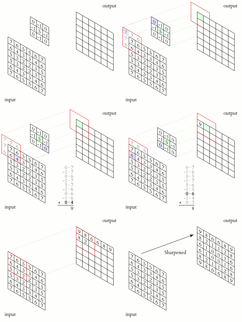
There are twos things to notice.

1. The signal convolving the 2D array is not the same as in our case. But the steps are the same, it’s just a different signal.
2. The values outside of the image are filled with 0s.

We can obtain the same behavior as 2. by using the np.pad function. It’s parameters are : the array / Image to pad, the padding size in 2D for the first and second axis, and the mode. The mode is the way we want to pad the image. We will use constant and set the value to 0.

 1
 2
 3
 4
 5
 6
 7
 8
 9
10

plt.imshow(img, cmap="grey")
plt.show()
img_padded = np.pad(img, [(1, 1), (1, 1)], mode="constant", constant_values=0)
img_smooth = np.zeros(img.shape)
for i in range(1, img.shape[0]):
    for j in range(1, img.shape[1]):
        img_smooth[i, j] = img[i-1 : i+1+1, j-1 : j+1+1].mean()

plt.imshow(img_smooth, cmap="grey")
plt.show()

The code is pretty straightforward:

• We start by copying the image and add padding,
• then for every pixel (i,j)
  1. We take a patch of size 3x3 centered on i,j using img[i-1 : i+1+1, j-1 : j+1+1]
  2. We compute the average of this patch and assign it to img_smooth[i,j].

I use j+1+1 because we want a patch from j-1 up to j+1 (included). But python indexing is exclusive on the upper bound.

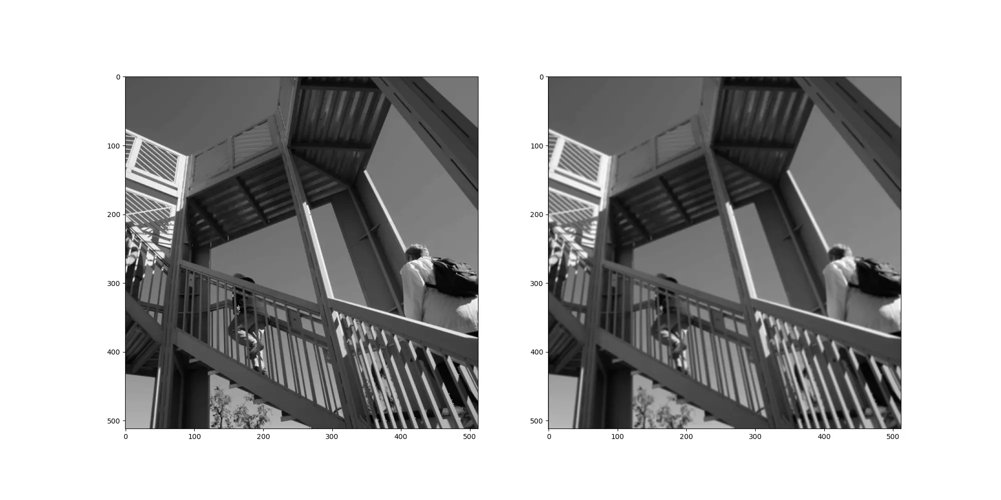
If you ran the code, you might have notice that it’s slow, and it’s normal, we are using not one but two for loops! And for loops are slow in python. It took: 667 ms ± 4.1 ms per loop (mean ± std. dev. of 7 runs, 1 loop each) using the for loop. How fast is it using a proper library ? Let’s use scipy.signal.convolve2D.

1
2
3

S = 3
img_smooth = sp.signal.convolve2d(img, np.ones(shape=(S, S)) / 9, mode="full")
# first signal is a 2D image and second is 3x3 signal of value 1/9

We simply convolve the image with a 3x3 signal of value 1/9.
Using scipy.signal.convolve2D it takes 1.72 ms ± 213 µs per loop (mean ± std. dev. of 3 runs, 1,000 loops each) a bit less than a 387x speedup !

Having fun with convolution and filters

One note before going on. From now on, I will call the first signal the image and the second one the “filter”

Back to our work, we can try to implement the difference between pixels using convolution! We need a signal that allows us to compute the difference between two pixels. At the beginning of this section we used [-1,1], but I want to change. Instead, we can use the following filter: \(B = [1, 0, -1]\). You might be thinking: “this means that we are subtracting the previous pixel to the following one”. And you’d be correct!
3 being odd, it allows to have a “center” in the patch. Which is useful when we want to assign the result of the convolution to the center pixel. Anyway, everyone uses the same filter and it’s a of size 3. Don’t hesitate to tell me if you know the real reason.
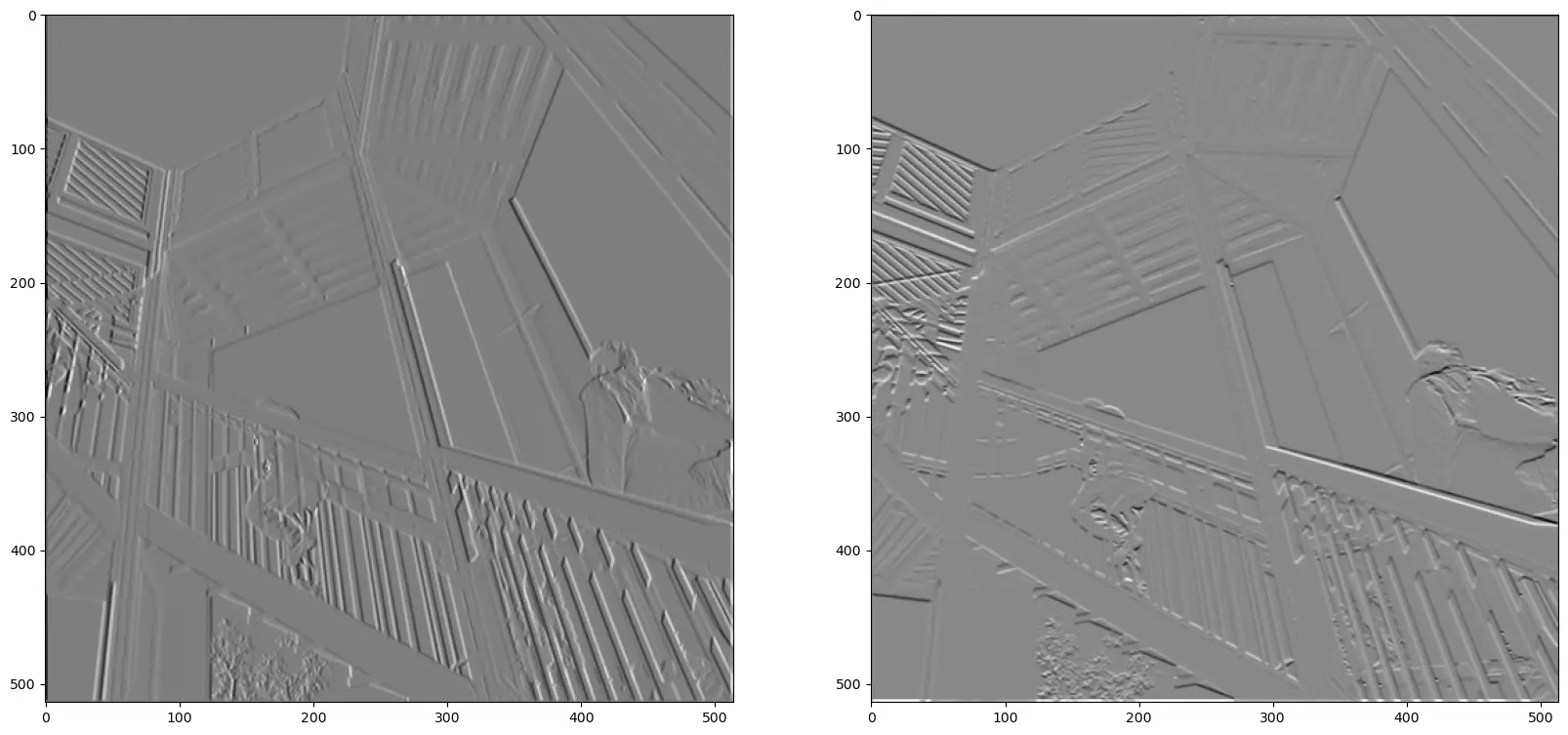
Now to the filter again. I hinted to use \(B = [1, 0, -1]\), what would it look like in 2D ? We can choose to apply the filter on the x axis or the y axis. Let’s try with x first, there exist mainly 3 filters to compute that : Prewitt, Sobel and Scharr. They are all 3x3 filters. And we can choose to apply them on the x or y axis simply by taking the transpose.

\begin{align} Prewitt &= \begin{bmatrix} -1 & 0 & 1 \\ -1 & 0 & 1 \\ -1 & 0 & 1 \\ \end{bmatrix} \\[20pt] Sobel &= \begin{bmatrix} -1 & 0 & 1 \\ -2 & 0 & 2 \\ -1 & 0 & 1 \\ \end{bmatrix} \\[20pt] Scharr &= \begin{bmatrix} -3 & 0 & 3 \\ -10 & 0 & 10 \\ -3 & 0 & 3 \\ \end{bmatrix} \end{align}

1
2
3
4
5
6
7

fig, ax = plt.subplots(1,2,figsize=(20,10))
sobel = np.array([[-1,0,1],[-2,0,2],[-1,0,1]])
img_sobel_x = sp.signal.convolve2d(img, sobel, mode="full")
# Notice the transpose used to make a derivative on the y axis
img_sobel_y = sp.signal.convolve2d(img, sobel.T, mode="full")
ax[0].imshow(img_sobel_x, cmap="grey")
ax[1].imshow(img_sobel_y, cmap="grey")

Toward a semantic analysis of images

We would like to have something a bit more abstract. Indeed, if we want to do something as simple as saying “are these two images showing the same scene ?” We need a way to compare them. And we can’t simply compare the pixel values, because if we take the same picture but with a different exposure from a different place, with more or less light, the pixel values will be different. We need to have a way to compare the content of the images. This is where the concept of features comes in. A feature is a part of the image that is interesting to us. It can be a corner, a line, a circle, etc. We can then compare the features of two images and say if they are similar or not just by comparing the features.

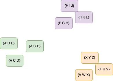
On the figure above, we see images with a label (the color). If we now extract the features {D F A} we could say that we are more likely green than purple. We can also say that we are more likely to be purple than red. This is the idea behind K-Nearest Neighbors. We compare our sample/image to the neighbors and take the label of the closest one. Given a new set of features (extracted from the images) we can compare them to our databases and try to find the closest images then get it’s label. We can therefore classify the new image.

How to detect similar images: The Harris corner detection algorithm

We can do exactly that and consider that we see an image through each feature. Let’s try to detect the corners and see if we can detect them after a rotation. We will use the Harris corner detection algorithm and then see how to implement it.

 1
 2
 3
 4
 5
 6
 7
 8
 9
10
11
12
13
14
15
16
17
18
19
20
21
22
23
24
25
26
27
28
29
30
31

rot = cv.getRotationMatrix2D((img.shape[0]//2, img.shape[1]//2), 30, 0.8)

img_rotated = cv.warpAffine(img, rot, img.shape)
fig, ax = plt.subplots(2,2,figsize=(20,20))
ax[0,0].imshow(img_rotated, cmap="gray")
ax[0,1].imshow(img, cmap="gray")

def draw_box(img, keypoints):
    kpts = keypoints
    img = cv.cvtColor(img, cv.COLOR_GRAY2RGB)
    img[kpts[0],kpts[1]+1] = [255,0,0]
    img[kpts[0],kpts[1]-1] = [255,0,0]
    img[kpts[0]+1,kpts[1]] = [255,0,0]
    img[kpts[0]-1,kpts[1]] = [255,0,0]
    img[kpts[0]+1,kpts[1]-1] = [255,0,0]
    img[kpts[0]+1,kpts[1]+1] = [255,0,0]
    img[kpts[0]-1,kpts[1]+1] = [255,0,0]
    img[kpts[0]-1,kpts[1]-1] = [255,0,0]
    return img

detection = cv.cornerHarris(img, 2, 3, 0.04)
dst = cv.dilate(detection,None)
detection2  = cv.cornerHarris(img_rotated, 3, 3, 0.04)
dst2 = cv.dilate(detection2,None)
id = np.array(np.where(dst>0.3*dst.max()))
id2 = np.array(np.where(dst2>0.4*dst2.max()))
img_corners = draw_box(img, id)
warped_corner = draw_box(img_rotated, id2)

ax[1,0].imshow(warped_corner)
ax[1,1].imshow(img_corners)

1. We start by rotating the image by 30 degrees and a scale of 0.8.
2. We then apply the Harris corner detection algorithm to both images.
3. We dilate the result to make the corners more visible.
4. We threshold the result to keep only the corners with a high response.
5. We then draw a box around the detected corners.

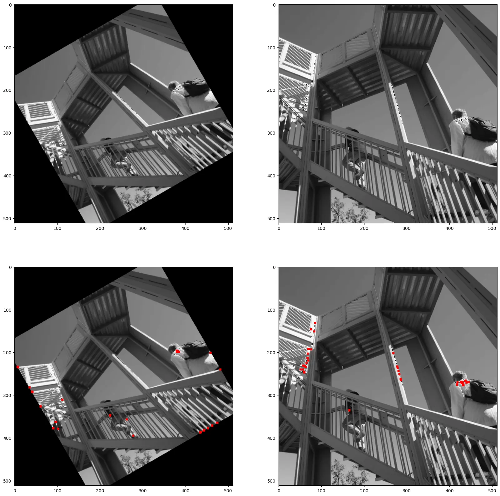
Not all corners are detected, furthermore some are detected in the original image but aren’t in the rotated one. We will see why when we implement it ourselves.

Now that we extracted the corners aka key points or interest points we can use them as features to compare images.

Conclusion

We’ve seen what a convolution is. How to implement the derivative of an images using them to highlight corners and edges on an images. Finally we used corners as features and I explained how to classify images using these features. An example of this will be available in the next part!
Stay tuned for part 2 !