Introduction

I’ve been studying ML for a few years, I mostly worked in PyTorch, but in recent years, I’ve heard a lot about Jax and I want to learn it. What better way than using it? In this blog post, we will speed run decades of machine learning by using automatic differentiation (Autodiff) in Jax. This allows us to take the derivative of computations expressed with Jax. Embark in this journey trough numeric differentiation and linear regression. In a second post we will continue with a much more advanced topic: building Meta’s LLM: Llama, a chatGPT competitor.

Prerequisite

Understanding of linear algebra and calculus is useful for the concepts presented here. If you are not familiar with these subjects, it might be challenging to follow along.

Gradient Descent & Supervised learning

The gradient descent is an optimisation process. We can use it to find the optimum of a function. Let’s say you have the function \(f(x) = x^2 \). We can find the minimum by following the slope. We know what the slope is, it’s the derivative evaluated at some point. Using the derivative, we can find an optimum (the minimum or maximum) Check the below gif to get an intuitive feeling.

Supervised learning use the above fact to find a parametrized function that give the correct results for a specific tasks. At first the function’s output is random. We compute the error between what we want and what our function predicts and we optimize the error to a minimum by changing the parameter of the function.

Here is an example: We have some training samples denoted \(\mathcal{X} = \{\mathcal{x_1} \dots \mathcal{x_n} \} \) and some corresponding outputs \(\mathcal{Y} = \{\mathcal{y_1} \dots \mathcal{y_n} \} \). We would like to find to find a function \(f \text{ such that } f(x_i) \approx y_i\). Let’s assume for our purpose that there exist a linear relationship between the input and the output. We would like to define \( f(x_i) = a\cdot x_i + b\) and find the values of \(a\) and \(b\). To do this we compute the error between the real value ( \(y_i\)) and our estimate of it (\(a\cdot x_i + b\)). The error is simply the substraction: \(y_i - (a\cdot x_i + b)\). We can now optimise this new expression with respect to a and b. i.e what are the a and b values that resutls in the lowest error. We can do that in Jax using the derivative (called the gradient if we are in more than 1 dimension)! Later in the text I will call them \(\beta_1 and \beta_0\)

Derivative with Jax.

Let’s start by simply taking a derivative using Jax. It allows us to express computations using Python and Jax. We can compile them to run on CPU, GPU, or TPU using XLA, this is a compiler for ML operation (i.e. matrix multiplication). The goal is to use the full potential of your hardware, but it also allows to compute derivative of our computations.

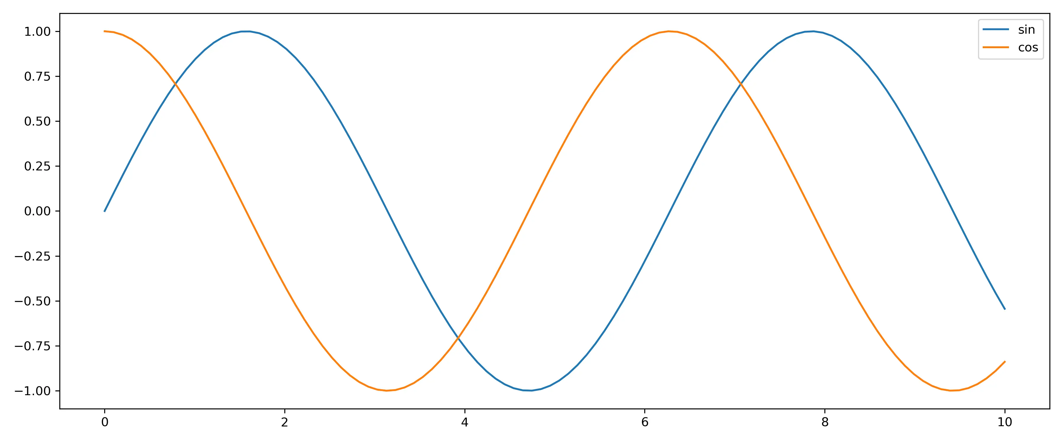
We will start slowly by taking the derivative of sine, which should be cosine.

 1
 2
 3
 4
 5
 6
 7
 8
 9
10
11
12
13
14
15
16

import jax.numpy as jnp
from jax import grad, vmap
import matplotlib.pyplot as plt
import seaborn as sns

X = jnp.linspace(0, 10, 100)
y_sin = jnp.sin(X)

cos = grad(jnp.sin)
y_cos = vmap(cos)(X)

# Plot using seaborn
fig, ax = plt.subplots(1,1, figsize=(12, 5))
sns.lineplot(x=X, y=y_sin, ax=ax,label="sin")
sns.lineplot(x=X, y=y_cos, ax=ax,label="cos")
plt.show()

The code is quite straightforward,

• We import our libraries.
• We create the X values and the corresponding y values of the sine function,
• We compute the cosine values.
• We show the plots.

The complicated lines are the computation of the cosine values.

 9
10

cos = grad(jnp.sin)
y_cos = vmap(cos)(X)

These two lines are the magic of Jax. We took the gradient (i.e. the derivative) of the sine function; this gives us the cosine function. But the grad function only applies to scalar functions. We could use a list comprehension [cos(x_val) for x_val in X] to evaluate the derivative for each x. But instead we use another tool in the Jax toolbox. vmap, this transforms a 1-to-1 function (taking 1 value and having 1 output) to taking n inputs and outputting n values. This is akin to calling the initial function multiple times. But vmap is highly efficient where the Python list comprehension isn’t! This is called vectorizing and is implemented using SIMD instruction in the CPU (it’s also optimized on GPU / TPU with other techniques)

When I said at the beginning that Jax was functional, it is because a lot of transformations take functions as input and output functions. You can clearly see it if you decompose vmap(cos)(X) into vect_cos_function = vmap(cos) and vect_cos_function(X).

The output of the above code is a graph showing both sine and its derivative, the cosine:

Linear Regression with Jax.

Ok, we now know how to use Jax to compute the gradient using jax.grad(fn) and vectorize a function using vmap. We have all we need to optimize a function. The idea is to follow the downward slope until you reach a minima of the function. (It can be a local one, which is not the best solution)

Let’s try to find a solution to the Linear Regression using Jax . In a simple (1 variable) linear regression , you have \(y_i = \beta_0 + \beta_1 \cdot x_i + \epsilon_i \) where each variable is a scalar. An example might help. Let’s say that \(y_i\) is the price of house \(i\) (out of N houses), \(\beta_0\) is a base price that every house is worth, while \(x_i\) is the area of house \(i\) (in \(\text{m}^2\)) and \(\epsilon \) is the error from the real price and our model. We would like to find the \(\beta\)’s.

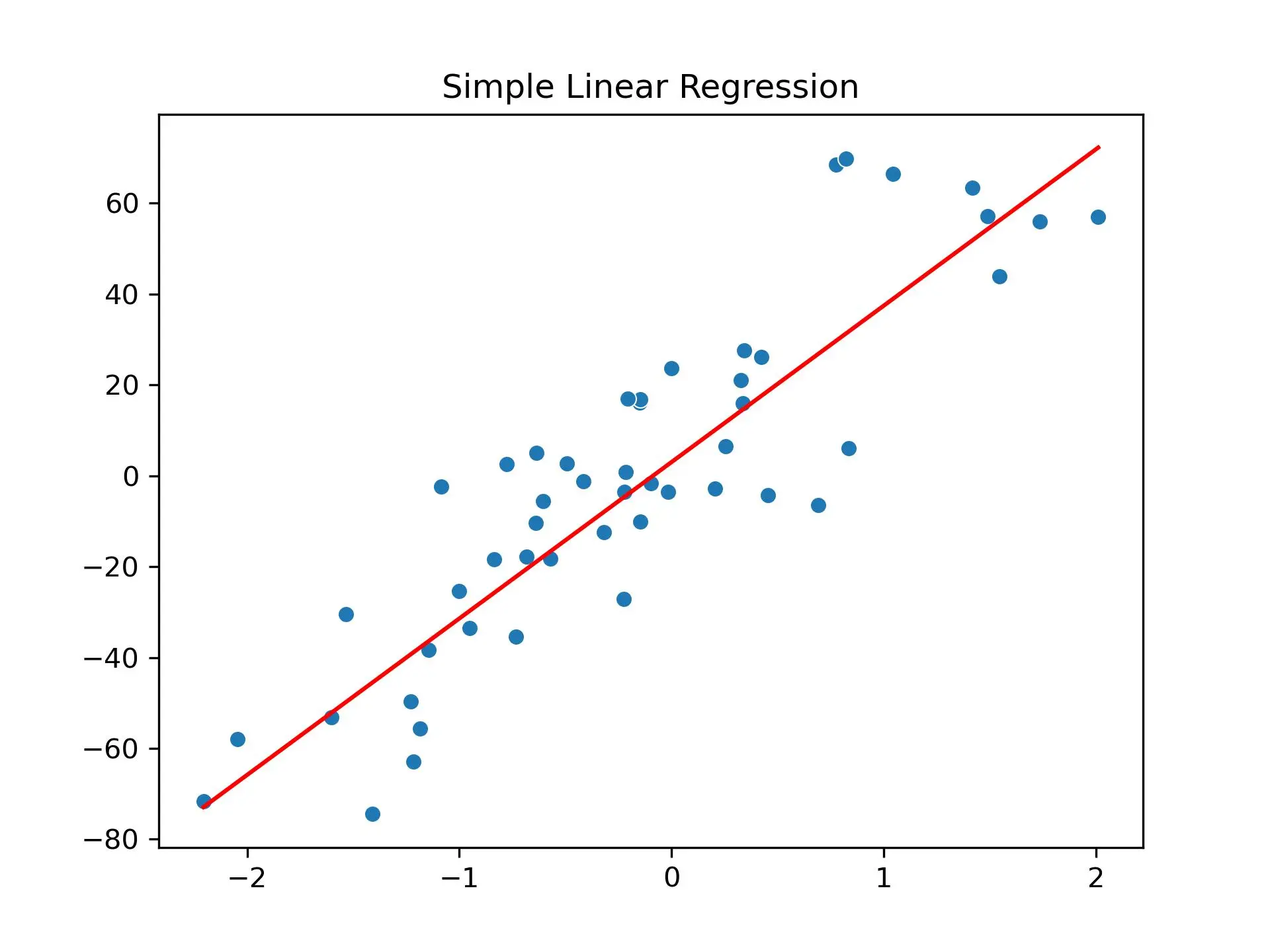
We start by creating a set of X,Y values following the above equation and we display both the points and the line.

 1
 2
 3
 4
 5
 6
 7
 8
 9
10
11
12

from sklearn.datasets import make_regression
b0 =3
X , y, coef = make_regression(n_samples=50,n_targets=1,n_features=1,noise = 20,bias=b0,coef=True,random_state=33)
X = X.reshape(-1) # reshape from (50,1) to (50,)
print(X.shape)
print(y.shape)
print(coef)
y_pred = coef * X + b0

ax = sns.scatterplot(x=X,y=y)
sns.lineplot(x=X, y= y_pred,color="red")
plt.title("Simple Linear Regression")

And this gives us:

We would like to find the b0 and the coef (the b1 in our math expression) automatically using Jax! We do it by computing an error between our prediction and the real value. The difference between the two is an error. We can minimise the error using the gradient descent and find a good solution.

 1
 2
 3
 4
 5
 6
 7
 8
 9
10
11
12
13
14
15
16
17
18
19
20
21
22
23
24
25
26
27
28
29
30
31
32
33
34
35

from sklearn.datasets import make_regression
from jax import vmap, grad
import seaborn as sns
from jaxtyping import Array, Float, PyTree

b0 = 3
X , y, b1 = make_regression(n_samples=50,n_targets=1,n_features=1,noise = 20,bias=b0,coef=True,random_state=33)
X = X.reshape(-1)

# compute the eror
def compute_error(b0: Float,b1: Float, x: Float[Array, "N"], y:Float[Array, "N"]):
    y_pred = b0 + b1*x
    return jnp.mean((y - y_pred)**2)

initial_b0 = jax.random.uniform(jax.random.key(42),shape=(1,)) # Chosen randomly
initial_b1 = jax.random.uniform(jax.random.key(42),shape=(1,)) # Chosen randomly
step_size = 0.001
for i in range(1000):
    grad_b0 = grad(compute_error,argnums=0)(initial_b0,initial_b1, X, y)
    grad_b1 = grad(compute_error,argnums=1)(initial_b0,initial_b1, X, y)
    # Notice how we update initial_b by SUBSTRACTING a fraction of the gradient.
    initial_b0 = initial_b0 - step_size*grad_b0
    initial_b1 = initial_b1 - step_size*grad_b1
    print(f"{initial_b0=}")
    print(f"{initial_b1=}")

print("Final values of b0 and b1:")
print(f"{initial_b0=}")
print(f"{initial_b1=}")
print("Optimal values of b0 and b1:")
print(f"b0: {b0}")
print(f"b1: {b1}")
ax = sns.scatterplot(x=X,y=y,color="blue")
sns.lineplot(x=X,y=initial_b0 + initial_b1*X, label="grad solution",ax=ax)
sns.lineplot(x=X,y=b0+ b1*X, label="optimal solution",ax=ax)

The code can look intimidating, don’t worry we will go through it.

1. We start by importing the lib.
2. We initialize the points for our regression, the X, y coordinates and we ensure that X has a shape of (n_samples,).
3. We define the compute_error function. This will give us a measurement of “how good we are”.

The complicated stuff is now the training loop where all the optimisations happens. We compute the derivative of the compute_error once with respect to b0 and once with respect to b1. Mathematically this is \( \frac{\partial \text{compute error}}{ \partial b_0} \) and \( \frac{\partial \text{compute error}}{ \partial b_1} \).

We can think of it as telling us how the error changes when we changes b0 by a tiny bit and this is the reason we can use the derivative to find values of b0 and b1 that yield a lower error.

18
19
20
21
22
23
24

step_size = 0.001
for i in range(1000):
    grad_b0 = grad(compute_error,argnums=0)(initial_b0,initial_b1, X, y)
    grad_b1 = grad(compute_error,argnums=1)(initial_b0,initial_b1, X, y)
    # Notice how we update initial_b by SUBSTRACTING a fraction of the gradient.
    initial_b0 = initial_b0 - step_size*grad_b0
    initial_b1 = initial_b1 - step_size*grad_b1

If you remember Figure1, we moved to a minimum by following the downward slope. The step_size in the above code is how much / how fast we are moving. grad(compute_error,argnums=0) computes the derivative of the compute_error function with respect to the \(0^{\text{th}}\) parameter and then we redo the same for the second (argnums=1) parameter.

The next point to notice is that updating the parameters (b0 and b1) is done by substracting a fraction of the gradients !

It makes sense, I’ll describe the 1D case and nD case. In 1D (Figure1) there are two cases:

1. We are after the minimum, aka where x > 0, in that area, the slope (derivative) is positive, and we want to go back, up to x = 0.
2. In the opposite case, where we are in the negative values of x, the slope (derivative) is also negative, and we want to go forward, towards x=0.

In both cases subtracting the derivative from x, takes us towards the minimum, notice that in our current example x is replaced with b0 and b1.

In higher dimension, we have that the directional derivative is maximal in the direction of the gradient, therefore we should take the opposite and we end up subtracting the gradient from the initial values to find a minimum. You can read this. if you want more details.

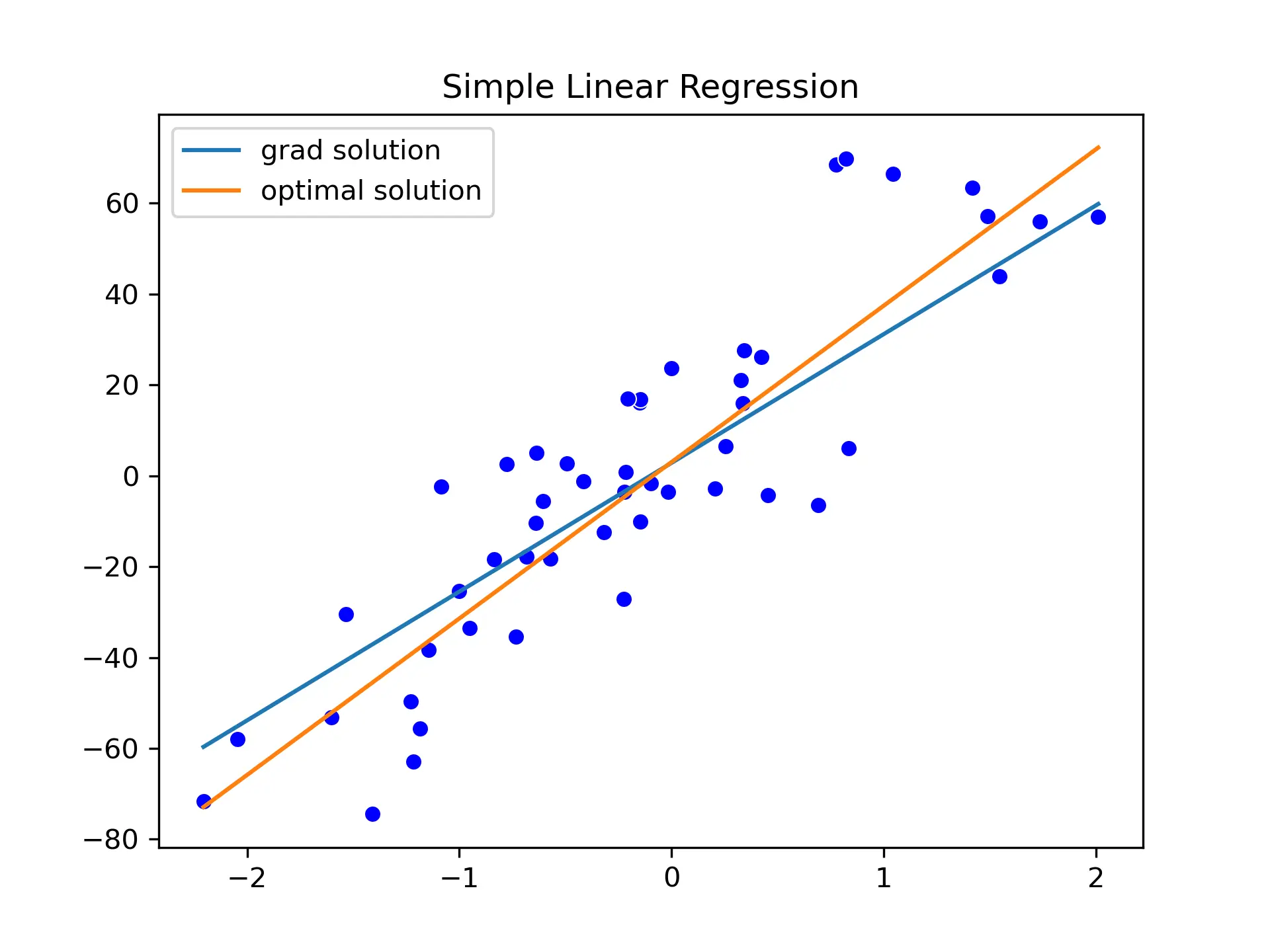
The output looks like that:

The values of b0 and b1 are slowly updated until we reach the b0=2.82435 and b1=28.328156. This is close to our optimal values of b0=3 and b1=34.41.

Going further

The optimal values of b0 and b1 are not of the same order of magnitude. Therefore, it might make sense to use a larger step_size for b1. This is where optimizers, come into play. They are used to efficiently update the parameters. Go take a look at

• adam
• adamw
• rmsprop

If you want to see how we can combine those building blocks to implement Llama, check my next article (to be published)